Computational Modeling

Much of the text shown on this page is taken from the author’s freely available article:

Brodland, G.W., 2015, "How computational models can help unlock biological systems," Seminars in Cell & Development Biology. doi:10.1016/j.semcdb.2015.07.001.

INTRODUCTION

Few things in the universe are as inspiring to behold as living systems, and one of the recurring mysteries about them is how their remarkable characteristics arise from interactions between relatively simple building blocks. For example, “How can collections of cells each of which is able to take only one of two states, on and off, allow human minds to think complex, meaningful thoughts?” or “How do the various organic and inorganic players in an ecosystem interact so as to produce long-term stability?” or “How do embryos acquire their increasingly complex and elegant forms?” These are profound mysteries.

As medical researchers and biologists strive to address questions of this kind with increasing rigour, they require tools that will allow them to gain insights into the complex interactions that occur in these systems, and one of the best currently-available tools is computational modeling [1-5]. There are many reasons that computational models are so effective in this setting, and a primary goal of this article is to highlight them, while at the same time recognizing their limitations. This article also aims to provide insight into how models work in general and show some of the specific ways that they can be used in the context of biological systems, especially those related to cell and tissue mechanics and embryology.

In general, the goal of a computational models is to replicate the behaviour of the systems they parallel and to do so based on actual, known properties of the system components. Achieving this goal may require the model to span a range of length scales and incorporate information from multiple fields of endeavour. As we will show, models that achieve this challenging goal can serve as an important complement to experimental and theoretical studies, and can provide valuable knowledge.

Before the advent of computers, one could write force balance equations describing equilibrium of forces at a single triple junction and volume constancy equations for single cells. However, studying interactions between meaningful numbers of cells by hand was impractical due to the large number of equations that had to be constructed and solved. To make matters worse, as the cells moved, their geometries changed and the equations had to be re-derived and re-solved for each small increment of motion.

When computers became available to university researchers in the early 1970s, they ushered in a revolution. With the advent of computers, code could be written to automatically construct and solve these equations and to do so repeatedly for multiple times steps. The time course of the cell movements could then be predicted and new things could be learned about how cells in model aggregates behaved [1]. Thus, computers provided a new way for researchers to investigate interactions between different systems elements.

Interest in the mechanics of cell-cell interactions was growing at the time, and there was debate about the nature of cellular forces and how they could drive collective phenomena such as cell sorting and aggregate rounding [6,7]. Some of the earliest computer programs were written to investigate the mechanics of cell-cell interactions and thereby tackle these intriguing questions. Even though many of those early studies were rudimentary by current standards, they were instrumental in defining the field of computational modeling and they unlocked important mysteries about how cells interact with each other [1].

Researchers quickly realized that they could change the properties of the virtual cells in their models and the rules that governed their interactionsat will, and that by doing so they could test hypotheses, understand which features gave rise to particular outcomes and carry out almost any kind of virtual experiment that crossed their minds. Over time, the algorithms they used improved and became more reliable, stronger connections were forged between models and real-world experiments, and modelling ultimately entered the mainstream of biology. Indeed, computational models have now become a standard tool for assessing proposed new biological mechanisms, often considered essential even when the associated experimental evidence is strong.

Many of the computational advances needed for these models came out of the fields of engineering and physics. The reason is that during the 1970s, 80s and 90s, computational models came to play an increasingly central role in various branches of engineering, especially its structural, aerospace, mechanical, electromagnetic, fluid dynamics, chemical, control and electrical domains [8]. It was in these contexts that extensive algorithm development took place and that the mathematical theory needed to bring confidence to the calculations was developed. In engineering and physics, a particular technique called the finite element method (FEM) took shape during this period and became the most widely-accepted, general-purpose framework for studying phenomena that involve non-trivial geometries. Many modern cell and tissue models, as well as other kinds of models, draw on conceptual and computational developments associated with this method.

A large variety of computational models arose for studying cells and their interactions during this time, including lattice (Potts), vertex, centric, and finite element models (reviewed by Brodland [1]), and since then, even more models have arisen [2,3,9-13]. Multiple approaches continue to be used because each one has its own inherent strengths and challenges. In addition, several large computational packages have become generally available, including CompuCell, The Virtual Cell and Smoldyn[14-16].

As this article discusses, computational models are based on specific conceptual, mathematical and algorithmic assumptions, and while these presuppositions can bring power and efficiency to the models, they can also introduce differences between the model and the real world that it endeavours to parallel.

Determining which model is most appropriate in a particular setting will depend on the focus and goals of the study, with options including deterministic versus stochastic approaches, agent (particle) versus continuum schemes, single- versus multiple-scale approaches and forward versus inverse approaches.

WHAT DOES IT MEAN TO MODEL SOMETHING?

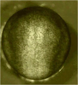
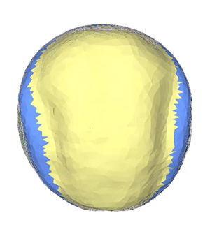
In order to better understand what it means to model something, consider Fig. 1, which shows a rectangular box across the top and represents the physical world, where a particular real embryo exists. For purposes of this illustration, we will consider the process of neurulation in amphibian embryos. An axolotl embryo at the start of this process is shown in the upper left corner of the figure. Over time, its neural plate, which consists of most of the visible tissue, rolls up to form a tube – the precursor of the spinal cord and brain – as shown in the other frames in the upper box. The box at the bottom represents the virtual or “in silico” world, and there one hopes that a corresponding model embryo is undergoing the same processes. Only when rendered using computer graphics does the model actually have any resemblance to the physical system it aims to represent, and when appropriately depicted, one hopes that it will appear very much like its archetype [17].

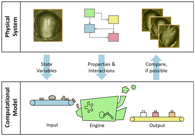
Figure 1 - The process of modelling. The rectangular box across the top represents the physical system while the lower box indicates the computational model. The arrows in between indicate how the state variables serve as input to the model while the properties and interactions instruct the function of the engine, where all calculations are done. The output of the engine is a set of numbers that can be rendered in various more readable forms and used to compare the model output with corresponding data in the physical system, where such exist. By comparing with physical data the model can be verified and validated (see text) and then used to predict behaviour where corresponding physical experiments may not exist, though care must be exercised if extrapolations are made.

At the moment shown, the embryo is generally spherical in shape, and its neural ridges, which trace an inverted U-shape around the upper (cephalic) three-quarters of the embryo and bound the neural plate, are just visible. Physical experiments carried out over several decades showed that a number of features of the embryo are crucial to its ongoing development. These include its current bulk and cellular geometries, the cellular architecture of its cytoskeleton and of other force generating systems, and the genes expressed in each cell and the proteins to which they have given rise [18-20]. It is generally understood that changes to any of these quantities would threaten the future of the embryo.

The in silico embryo must match at least these features, and we call the numbers or other quantitative descriptors that embody them “state variables” because they describe the current state of the model embryo. An important part of the modeling process is to choose these state variables well. The set must include all quantities important to the embryo during the period to be modelled, but not be encumbered by too many unnecessary ones. Proper choice of these variables requires a certain amount of prior understanding of the system of interest. Measured or estimated values of these state variables – which in the case of the embryo shown included thousands of surface points that defined the exterior form of the embryo, gene expression patterns, cytoskeletal morphologies, and cell fabric (size, shape and directionality) information – serve as the input to the computational model.

Over time, the physical features of the embryo as captured by its state variables interact with each other, producing a specific change in the geometry of the embryo, hopefully the one necessary to form properly its neural tube. The model must simulate these interactions – some of which, like tissue force-elongation relationships, can be captured in the form of material properties [21]. The purpose of the computational “engine” is to faithfully reproduce these interaction using mathematical relationships and computational algorithms. In order to do this, most engines use the mathematical machinery developed for a particular approach – such as a finite element or Potts method – but sometimes custom approaches are used [9,10,22]. Much of the success of a model can depend on choosing an appropriate engine, and fine tuning its operational parameters, such as the size of the time step used for a particular simulation. Although some of the powerful commercial finite element packages may seem suitable for cell studies, they do not generally tolerate negative stiffnesses which some cellular components exhibit [1], nor are they designed to accommodate biologically-distinctive features such as cells or their neighbour changes [23].

As the engine runs, it reports the results of its calculations, which may include the current locations of all of the points used to define its geometry, regional cellular fabric (size, shape and directionality), internal stress values, and updated cytoskeletal and genomic information. Suitable graphics routines are essential for transforming the numerical findings into a more comprehensible form. The various components of the output can be compared to any corresponding values that are known for the physical system. If there is good agreement, it indicates that the chosen state variables and interactions are sufficient to explain the observed phenomenon. Unfortunately, agreement does not prove that the mechanism embodied in the model is the only possible explanation. In contrast, lack of agreement indicates that the variables and interactions assumed in the model are not sufficient to account for the physical observations. This outcome often gives rise to further thought, additional physical or numerical experiments, revised models and, hopefully, new understanding.

A broad range of factors can be considered in making these comparisons. In the model of neurulation discussed here, these comparisons included bulk tissue motions, regional strain rate profiles, maps of tissue stresses, tissue thicknesses and cross-sectional silhouettes, and cell shape details [21,24]. In other kinds of biological systems, one might consider factors such as stochastic fluctuations, system stability, time constants,phase transitions, bifurcations, or signatures that are useful for classifying system behaviour.

WHAT OUR MODEL OF NEURULATION SHOWED US

(This section is NOT from the Seminars in Cell & Development Biology article.)

One of the critical patterns of tissue motion that occurs in all vertebrates is called neurulation (Video 1). It involves a sheet of tissue rolling up into a tube that is the precursor of the spinal cord and the brain. If part of the tube does not close, a serious birth defect (such as spina bifida or anencephaly) can result.

In order to figure out the forces that drive neurulation (Video 1),we built a 3D model and adjusted its driving forces until the motions it produced(Video 2) matched those in the real embryo [21,24]. The motions that the model generated were highly sensitive to details of the applied forces, and so when the model tissue motions matched those in real embryos, onesome confidence that the driving forces were correct. To further verify the driving forces, we ensured that the cell shapes, strain rates and tissue thicknesses predicted by the model matched those present in real embryos.

Various genetic mutations were believed to affect particular sub-cellular force-generating structures and when the driving forces in the model were adjusted in accordance with those expectations, the model produced malformations (Figure 2) that agreed well with those found in mutant embryos. The model was thus able to verify how specific genes affect the microscopic force generating structures in the cells, how these changes affect the forces in cells and tissues, how these force alterations affect tissue movements, and how they ultimately determine whether the final embryo shape is normal or not [21, 24]. One of the surprising findings of the study was that changing the driving forces by as little as 20% can give rise to malformations (birth defects).

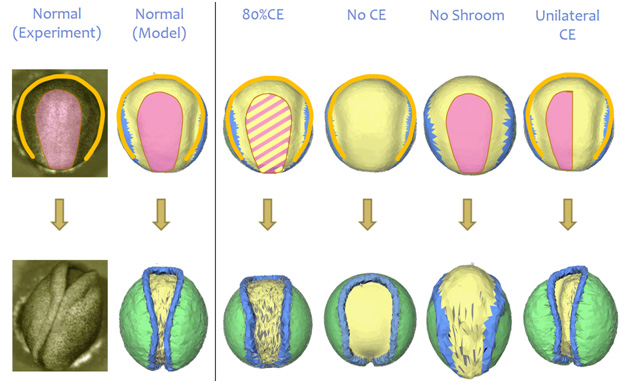
Figure 2 – Changing the driving forces in the model in various ways gave rise to defects (malformations) that were consistent with those observed in real embryos [21,24].

IN SUMMARY

One of the overarching reasons that models can help to unlock biological systems is that they offer perspectives different than those provided by experiments and theory. Science could advance without models, but progress would be considerably slower and more circuitous, just as it would be if experiments or theory were not available. Models have value because they allow their users to peer at deadbolt mechanisms from a different vantage point, sometimes even from inside. The additional knowledge and new perspectives they bring are often enough when added to experimental and theoretical contributions to allow the bolt to finally be drawn back and the door that barred a previously-hidden vista to finally be pushed open.

References

[1] GW Brodland. Computational modeling of cell sorting, tissue engulfment, and related phenomena: A review, ApplMech Rev. 57 (2004) 47-76.

[2] MRK Mofrad, RD Kamm, Cytoskeletal mechanics: models and measurements, Cambridge University Press, Cambridge ; New York, 2006.

[3] A Chauvière, L Preziosi, C Verdier, Cell mechanics: from single scale-based models to multiscale modeling, Chapman & Hall/CRC, Boca Raton, FL, 2010.

[4] Y Kam, KA Rejniak, AR Anderson. Cellular modeling of cancer invasion: integration of in silico and in vitro approaches, J.Cell.Physiol. 227 (2012) 431-438.

[5] ARA Anderson, MAJ Chaplain, KA Rejniak, Single-cell-based models in biology and medicine, Birkhäuser, Basel ; Boston, 2007.

[6] MS Steinberg. Does differential adhesion govern self-assembly process in histogenesis? Equilibrium configurations and the emergence of a hierarchy among populations of embryonic cells, J Exp Zool. 173 (1970) 395-434.

[7] AK Harris. Is cell sorting caused by differences in the work of intercellular adhesion? A critique of the steinberg hypothesis, J.Theor.Biol. 61 (1976) September.

[8] OC Zienkiewicz, RL Taylor, The Finite Element Method for Solid and Structural Mechanics, Elsevier, Oxford, 2005.

[9] SA Sandersius, TJ Newman. Modeling cell rheology with the Subcellular Element Model, Phys.Biol. 5 (2008) 015002.

[10] T Kim, ML Gardel, E Munro. Determinants of fluidlike behavior and effective viscosity in cross-linked actin networks, Biophys.J. 106 (2014) 526-534.

[11] IM Gemp, RW Carthew, S Hilgenfeldt. Cadherin-dependent cell morphology in an epithelium: constructing a quantitative dynamical model, PLoSComput.Biol. 7 (2011) e1002115.

[12] H Honda, T Nagai. Cell models lead to understanding of multi-cellular morphogenesis consisting of successive self-construction of cells, J.Biochem. 157 (2015) 129-136.

[13] R Magno, VA Grieneisen, AF Maree. The biophysical nature of cells: potential cell behaviours revealed by analytical and computational studies of cell surface mechanics, BMC Biophys. 8 (2015) 8-015-0022-x. eCollection 2015.

[14] M Swat, GL Thomas, JM Belmonte, A Shirinifard, D Hmeljak, JA Glazier. Multi-Scale Modeling of Tissues Using CompuCell3D, Methods in Cell Biology. 110 (2012) 325-366.

[15] DC Resasco, F Gao, F Morgan, IL Novak, JC Schaff, BM Slepchenko. Virtual Cell: computational tools for modeling in cell biology, Wiley Interdiscip.Rev.Syst.Biol.Med. 4 (2012) 129-140.

[16] M Robinson, SS Andrews, R Erban. Multiscale reaction-diffusion simulations with Smoldyn, Bioinformatics. (2015).

[17] GJ Bootsma, GW Brodland. Automated 3-D reconstruction of the surface of live early-stage amphibian embryos, IEEE Trans Bio-Med Eng. 52 (2005) 1407-1414.

[18] T Mammoto, A Mammoto, DE Ingber. Mechanobiology and developmental control, Annu.Rev.CellDev.Biol. 29 (2013) 27-61.

[19] S Kim, PA Coulombe. Emerging role for the cytoskeleton as an organizer and regulator of translation, Nat.Rev.Mol.Cell Biol. 11 (2010) 75-81.

[20] B Alberts, D Bray, K Hopkin, A Johnson, J Lewis, K Roberts, et al., Essential cell biology. 4th Edition, Fourth ed., Garland Publishing Inc., New York, 2014.

[21] X Chen, GW Brodland. Multi-scale finite element modeling allows the mechanics of amphibian neurulation to be elucidated, Physical Biology. 5 (2008) 015003.

[22] DB Staple, R Farhadifar, JC Roper, B Aigouy, S Eaton, F Julicher. Mechanics and remodelling of cell packings in epithelia, Eur.Phys.J.E.Soft Matter. 33 (2010) 117-127.

[23] HH Chen, GW Brodland. Cell-level finite element studies of viscous cells in planar aggregates, J BioMech Eng. 122 (2000) 394-401.

[24] GW Brodland, X Chen, P Lee, M Marsden. From genes to neural tube defects (NTDs): insights from multiscale computational modeling, HFSP J. 4 (2010) 142-152.